AI Model Drift Detection and Retraining: Maintenance Guide for Production ML Systems

A landmark MIT research study examining 32 datasets across four industries revealed a sobering reality: 91% of machine learning models experience degradation over time. Even more concerning, 75% of businesses observed AI performance declines without proper monitoring, and over half reported measurable revenue losses from AI errors. When models left unchanged for six months or longer see error rates jump 35% on new data, the business impact becomes impossible to ignore. 

This is the reality of production AI maintenance. Unlike traditional software, which remains static until you explicitly change it, machine learning models exist in a state of continuous silent degradation. The data they encounter in production differs from their training data. User behaviors evolve. Market conditions shift. Regulatory environments change. Each of these forces creates AI model drift detection challenges that require systematic, ongoing management. 

Organizations that implement robust model performance monitoring, establish clear retraining triggers, and automate their ML retraining schedule maintain accurate, valuable models throughout their production lifetime. These organizations gain competitive advantage not through having better models initially, but through maintaining better models continuously. 

This comprehensive step-by-step guide walks you through the complete framework for detecting model drift, deciding when to retrain, implementing automated retraining pipelines, and establishing sustainable AI system upkeep practices. Whether you’re managing recommendation systems, fraud detection, predictive analytics, or any other ML application, this guide provides actionable strategies tested in production environments managing millions of predictions daily.  

Understanding Model Drift: Why Your Production Models Fail Over Time 

What Is Model Drift? The Phenomenon Destroying Your ML ROI 

AI model drift detection begins with understanding exactly what drift is and why it matters. Model drift, also called model degradation or AI aging, refers to the gradual (or sometimes sudden) decline in a model’s predictive accuracy and business value over time. Unlike other software failures, model drift often occurs silently, without errors or exceptions. Your model continues to make predictions. It continues to run. Yet its predictions become progressively less accurate or relevant. 

Consider a concrete example: A bank trained a credit risk model using three years of customer data from 2021-2023. The model performed excellently, correctly identifying 95% of default risk. The bank deployed it into production in January 2024.

By September 2024, the same model was only identifying 87% of defaults correctly. Nothing in the code has changed. The model continued running exactly as it was deployed. But the model’s performance degraded 8 percentage points because economic conditions changed, customer behavior evolved, and new types of credit risk emerged that the training data had never encountered. 

This model drifts in its most common form. And it’s why production of AI maintenance isn’t optional; it’s essential. 

Data Drift vs. Concept Drift: Two Different Problems Requiring Different Solutions 

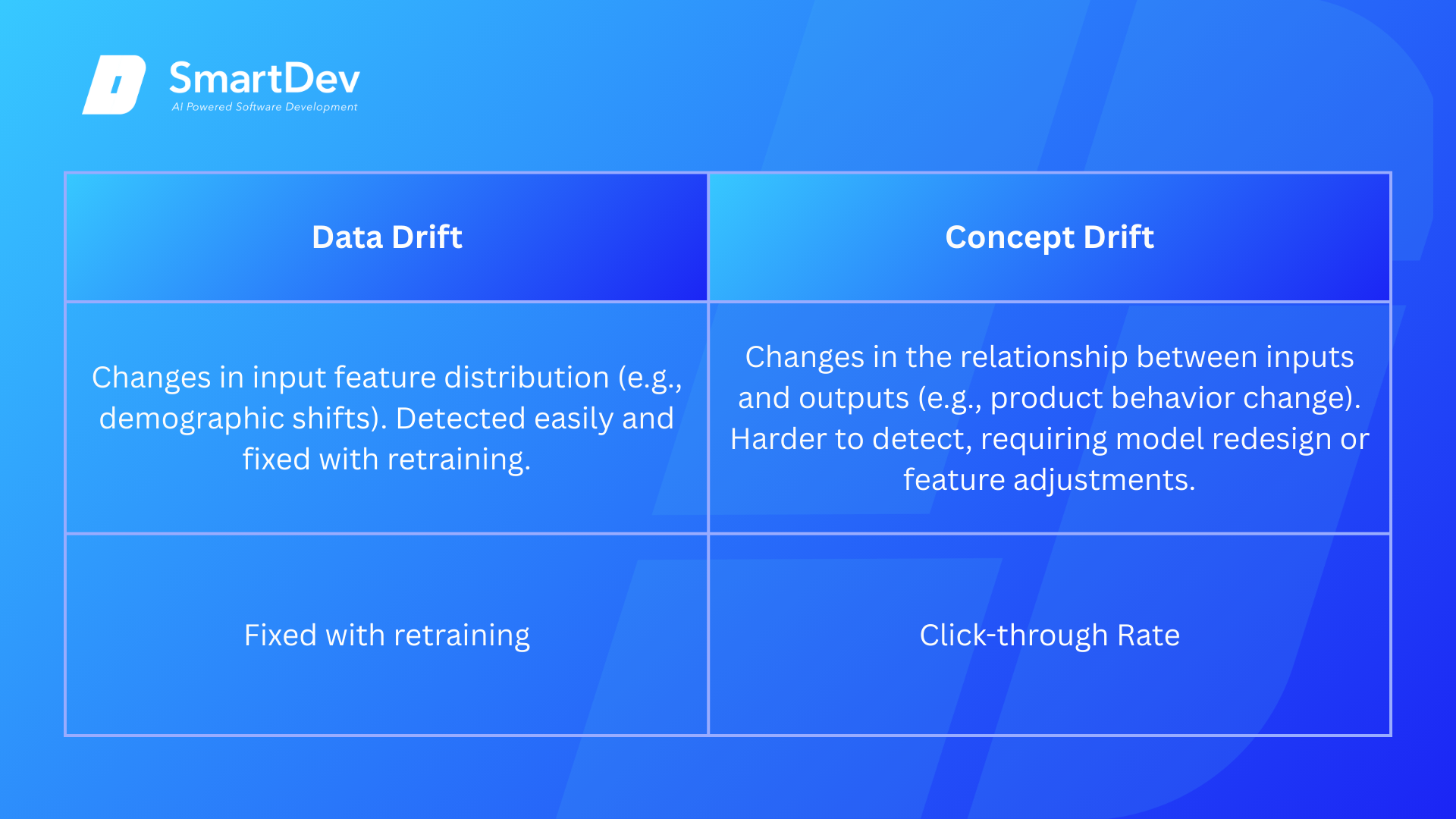
Understanding AI model drift detection requires distinguishing between two fundamentally different failure modes: data drift and concept drift. They sound similar, but they create different problems and require different solutions. 

Data drift (also called covariate shift or feature drift) occurs when the statistical distribution of input features changes relative to the training data distribution. Imagine you built a model predicting customer purchasing behavior based on age, income, location, and browsing history. Your training data showed that 60% of customers aged 25-40.

But in production, the customer’s demographic shifts, now only 30% are in that age range. The relationship between age and purchasing behavior hasn’t changed. The definition of “customer” hasn’t changed. But the distribution of ages has shifted. This is a data drift. 

Data drift is relatively straightforward to detect and handle. You can measure statistical changes in input distributions using techniques like Population Stability Index (PSI), Kolmogorov-Smirnov tests, or Jensen-Shannon divergence. Often, retraining your model on recent data with the new distribution is sufficient to restore performance. 

Concept drift is fundamentally different and more insidious. Concept drift occurs when the relationship between input features and target variables fundamentally changes. The underlying concept your model learned no longer applies. Perhaps you built a model predicting customer churn. Your training data showed that customers who don’t log in for 30 days are likely to cancel.

But the product changed customers can now accomplish key tasks via mobile app notifications without logging into the web platform. So, customers who don’t log in aren’t necessarily churning. The relationship between logging in and churn has fundamentally changed. 

Concept drift is harder to detect because the input data distribution may look unchanged. You need different monitoring approaches – monitoring whether model outputs are still aligned with business outcomes, checking if certain feature-target relationships have broken down, or monitoring prediction distributions to see if your model’s confidence levels have become miscalibrated. 

This distinction matters enormously for your ML retraining schedule. Simple data drift can often be addressed through periodic retraining on recent data. Concept drift may require model redesign, feature engineering changes, or even fundamental rethinking of the problem. 

The Business Impact of Untreated Model Drift 

Ignoring model drift isn’t just a technical problem; it’s a business problem. The costs accumulate quickly: 

• Immediate revenue impact: Recommendation systems showing wrong products reduce click-through rates and average order value. Fraud detection models missing fraud led to direct losses. Pricing models that make suboptimal decisions reduce margins. Lead scoring models misdirecting sales efforts waste high-value sales time. 

• Customer experience degradation: Users notice when recommendations become irrelevant, when customer service chatbots give wrong information, and when personalization disappears. These experiences damage brand perception and increase churn. 

• Compliance and regulatory risk: Models used for hiring, lending, or other consequential decisions must maintain fairness and explainability. As models degrade, fairness metrics often break down. A model that was 95% accurate across demographic groups might become 85% accurate for minority groups, creating legal and regulatory exposure. 

• Operational costs: Without automation, maintenance becomes expensive. Data scientists spend time debugging degraded models, manually retraining, testing new versions, and deploying fixes. Organizations without proper model performance monitoring often discover problems weeks or months after they’ve started costing money. 

The MIT study on model degradation found that different models degrade at dramatically different rates on the same data. Some models degrade gradually and predictably. Others experience “explosive degradation” – performing well for an extended period, then suddenly collapsing. Without proper monitoring, you won’t know which pattern your model exhibits until it’s too late. 

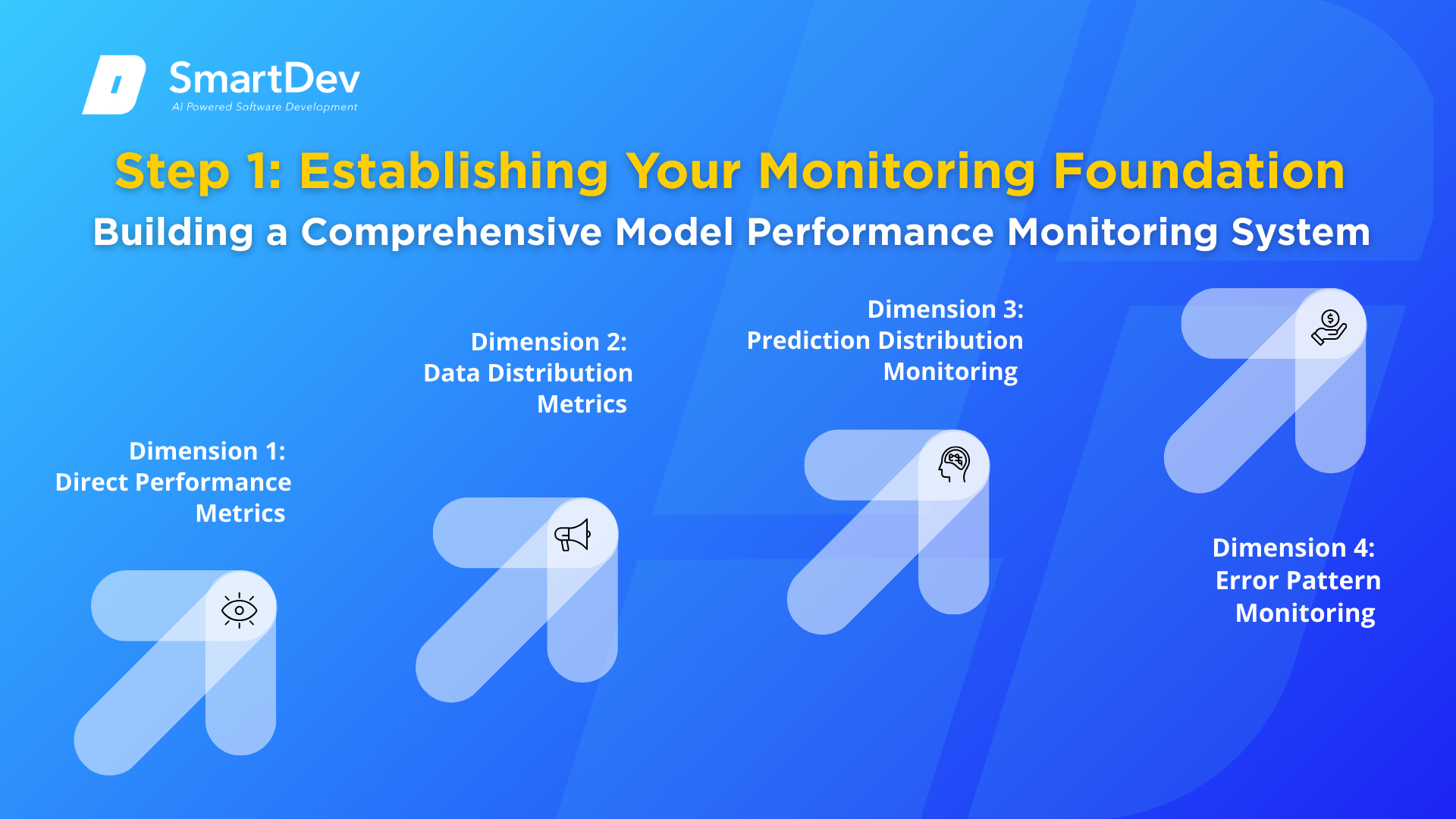
Step 1: Establishing Your Monitoring Foundation 

Building a Comprehensive Model Performance Monitoring System 

The foundation of effective AI model drift detection is comprehensive model performance monitoring. This isn’t optional – it’s the prerequisite for everything else. Without monitoring, you cannot detect drift, decide when to retrain, or know if your retraining worked. 

Your production AI maintenance monitoring system should track metrics across four dimensions: 

Dimension 1: Direct Performance Metrics 

These are the metrics that directly measure whether your model is solving its intended problem. For a classification model, this might be accuracy, F1-score, precision, recall, AUC-ROC, or the Gini coefficient. For regression, it might be RMSE, MAE, R-squared, or MAPE. For ranking systems, NDCG or average precision. 

The critical principle: measure what matters to your business, not just what’s easy to measure. If your fraud detection system catches 99% of fraud but takes a week to investigate alerts, that high accuracy creates business value only if the investigation is fast. Your monitoring should track both the detection rate and the investigation time. 

Implement these monitoring practices: 

• Calculate metrics daily or in real-time depending on your prediction volume. 

• Segment metrics by cohort (e.g., by geography, customer segment, product category). A model’s overall accuracy might be stable while performance for specific segments collapses. 

• Track percentile metrics: Don’t just track average performance. Track 25th, 50th, and 75th percentile performance. MIT research found that while median performance appeared stable, the gap between best-case and worst-case performance increased over time; indicating the model was becoming unreliable. 

• Establish rolling baselines: Calculate baseline performance over a 15-30 day stable production window. Then compare current performance against that baseline. 

Dimension 2: Data Distribution Metrics 

Since labeled data often arrive with delay, you need proxy metrics that detect changes in input data distribution; warning signs that performance degradation is likely coming even before you can directly measure it. 

Key techniques: 

• Population Stability Index (PSI): Measures how much a feature’s distribution has changed from training. Calculate for each important feature. PSI values over 0.25 warrant investigation; values over 0.1 warrant attention 

• Kolmogorov-Smirnov (KS) Test: Compares observed feature distributions to training distributions 

• Jensen-Shannon Divergence: Measures divergence between training and production feature distributions 

• Feature-specific monitoring: Track mean, standard deviation, min, max, and quartiles for each numerical feature

Implement these checks: 

• Run daily distribution comparisons 

• Set alerts for features exceeding predefined divergence thresholds 

• Track divergence trends – increasing divergence over time suggests growing data drift 

Dimension 3: Prediction Distribution Monitoring 

Beyond input features, monitor what your model is actually predicting. Changes in prediction distributions can signal that your model is encountering data outside its training distribution. 

Key metrics: 

• Prediction distribution shifts: Compare the distribution of predicted values in production versus what was observed during training. Large shifts suggest the model is encountering scenarios it wasn’t trained for. 

• Confidence calibration: If your model outputs prediction probabilities, monitor whether they remain well-calibrated. A model that predicts 90% confidence should be correct roughly 90% of the time. Degrading calibration indicates model uncertainty about data it’s encountering. 

• Prediction stability: Models should produce relatively stable predictions from week to week (accounting for seasonality). Erratic prediction changes without corresponding data changes suggest instability. 

Dimension 4: Error Pattern Monitoring 

Analyzing how your model fails reveals important information about what’s changing: 

• Error distribution: Track not just error rate, but types of errors. Different error types suggest different root causes. 

• Temporal error patterns: Are errors increasing uniformly or concentrated in specific time periods? Concentrated errors might indicate environmental changes (new competitors, regulatory changes, seasonal shifts) 

• Feature-specific error patterns: Which features are involved in predictions where the model fails? Feature-specific errors suggest specific features have drifted. 

Setting Up Your Monitoring Infrastructure 

Practical implementation approaches: 

Option 1: DIY with Open Source 

• TensorFlow Data Validation (TFDV): Statistical validation and drift detection 

• Evidently AI: Comprehensive monitoring dashboards and alerts 

• Prometheus + Grafana: Time-series monitoring and visualization 

• Custom Python scripts processing daily prediction logs 

• Cost: Primarily engineering time to implement and maintain 

Option 2: Specialized ML Monitoring Platforms 

• Arize AI, Datadog ML Monitoring, WhyLabs, Amazon SageMaker Model Monitor 

• Provide pre-built dashboards, alert systems, and specialized metrics 

• Often integrate with model registries and deployment pipelines 

• Cost: Platform subscription ($2,000-$20,000+ per month depending on scale) but reduced engineering overhead 

Option 3: Hybrid Approach
Most production systems combine approaches: open source for custom metrics and specific business logic, commercial platforms for standard monitoring and alerting. 

Step 2: Detecting Model Drift: Recognizing When Your Model Is Failing 

Implementing Automated Drift Detection Signals 

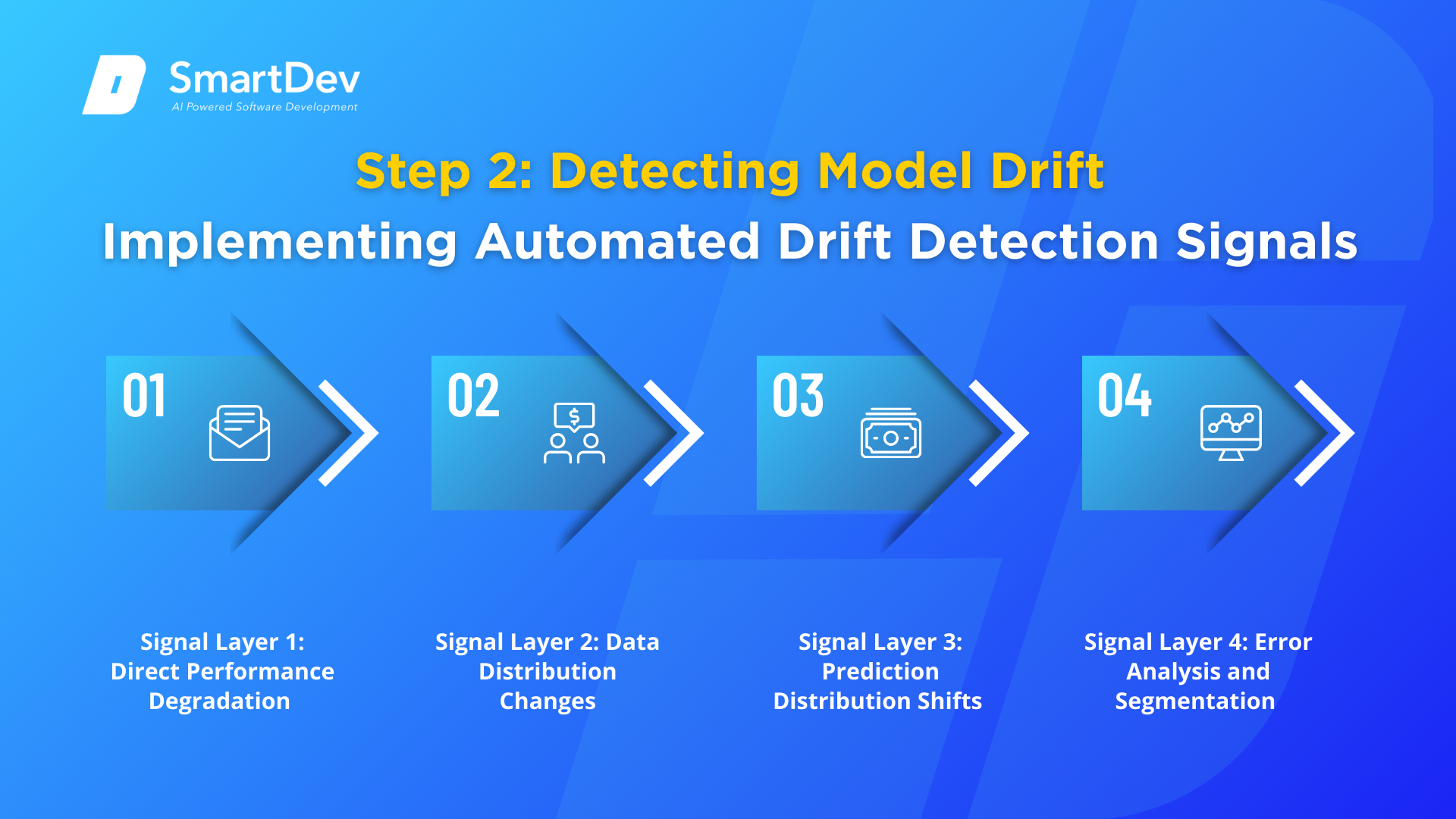
Detecting model drift requires combining multiple signals. No single metric perfectly identifies when retraining is needed. Instead, implement a layered approach where multiple signals increase confidence that drift has occurred. 

Signal Layer 1: Direct Performance Degradation 

The most important signal: your model’s performance metrics have declined. 

Implementation: 

• Daily calculation of primary performance metric 

• Comparison against rolling baseline (typically 30-day rolling average or percentile benchmark) 

• Trigger alert when primary metric drops below threshold (typically 1-3% degradation) 

• Segment by important cohorts – sometimes overall metric looks stable but specific segments degrade severely 

Example trigger logic: 

A recommendation system might trigger alerts when: 

• Overall click-through rate drops 2% from baseline, OR 

• Click-through rate for new users (acquired in past 30 days) drops 5% from baseline, OR 

• Click-through rate for a specific product category drops 4% from baseline 

Signal Layer 2: Data Distribution Changes 

When you can’t wait for labeled data, distribution changes provide early warning signs. 

Implementation: 

• Calculate PSI for important features daily 

• Set thresholds: investigate PSI > 0.1, alert PSI > 0.25 

• Track trends-gradually increasing PSI indicates creeping drift; sudden jumps indicate sudden changes 

• Compare recent production data against training data distribution 

Example detection: 

A churn prediction model might detect: 

• Customer age distribution changing (younger customers increasing) 

• Subscription contract term distribution changing 

• Usage pattern distribution changing 

Interpretation: These distribution changes indicate that the customers the model is scoring are different from the customers it was trained on. Model retraining may be needed. 

Signal Layer 3: Prediction Distribution Shifts 

When model output distributions change significantly from training, the model is scoring different data. 

Implementation: 

• Calculate prediction distribution statistics weekly (mean, std dev, percentiles) 

• Compare against training period baseline 

• Investigate when 25th percentile prediction drops significantly (model becoming less confident) 

• Monitor for prediction values outside training range 

Example: 

A price optimization model trained on laptops priced $500-$3,000 is now trying to price laptop bundles priced $1,500-$8,000. The prediction distribution shifts dramatically-the model is outside its training distribution. 

Signal Layer 4: Error Analysis and Segmentation 

Dig deeper into how your model fails: 

Implementation: 

• Weekly review of highest-error predictions 

• Segment errors by feature value ranges 

• Identify whether errors concentrate in specific scenarios 

• Compare error patterns to previous periods 

Example: 

A fraud detection model detecting increased false negatives specifically for transactions involving new merchants suggests fraudsters have changed their tactics to include merchants the model wasn’t trained on. 

Establishing Drift Detection Thresholds 

A critical and often overlooked step: determining what constitutes “drift that requires action.” 

Too-strict thresholds cause false alarms. You retrain constantly, waste resources, introduce deployment risk unnecessarily, and potentially make things worse. 

Too-loose thresholds cause missed drift. You continue deploying a degraded model while paying the business cost of poor predictions. 

Framework for Setting Thresholds:

1. Establish baseline during stable period: Deploy your model, allow 2-4 weeks of stable production, then measure baseline performance and data distributions. This period should be representative of typical operating conditions.

2. Understand costs and benefits:

• Cost of retraining: Infrastructure costs, engineering time, deployment risk 

• Cost of model degradation: Business impact of inaccurate predictions, customer dissatisfaction 

• For high-impact models (fraud detection, medical diagnosis), lower thresholds are justified 

• For low-impact models (non-critical recommendations), higher thresholds may be acceptable

3. Set initial thresholds conservatively: Start with thresholds requiring clear, unambiguous degradation before triggering retraining. Adjust tighter or looser based on experience.

4. Consider trend thresholds: Don’t just alert to absolute degradation. Alert on direction and rate of change:

• Gradual degradation of 0.5% per week → alert if continues 4 weeks 

• Sudden 5% degradation → alert immediately 

• This approach catches creeping drift earlier while avoiding false alarms from normal noise 

5.  Segment-specific thresholds: Different business segments may warrant different thresholds. High-value customer segments might warrant more aggressive retraining than low-value segments.

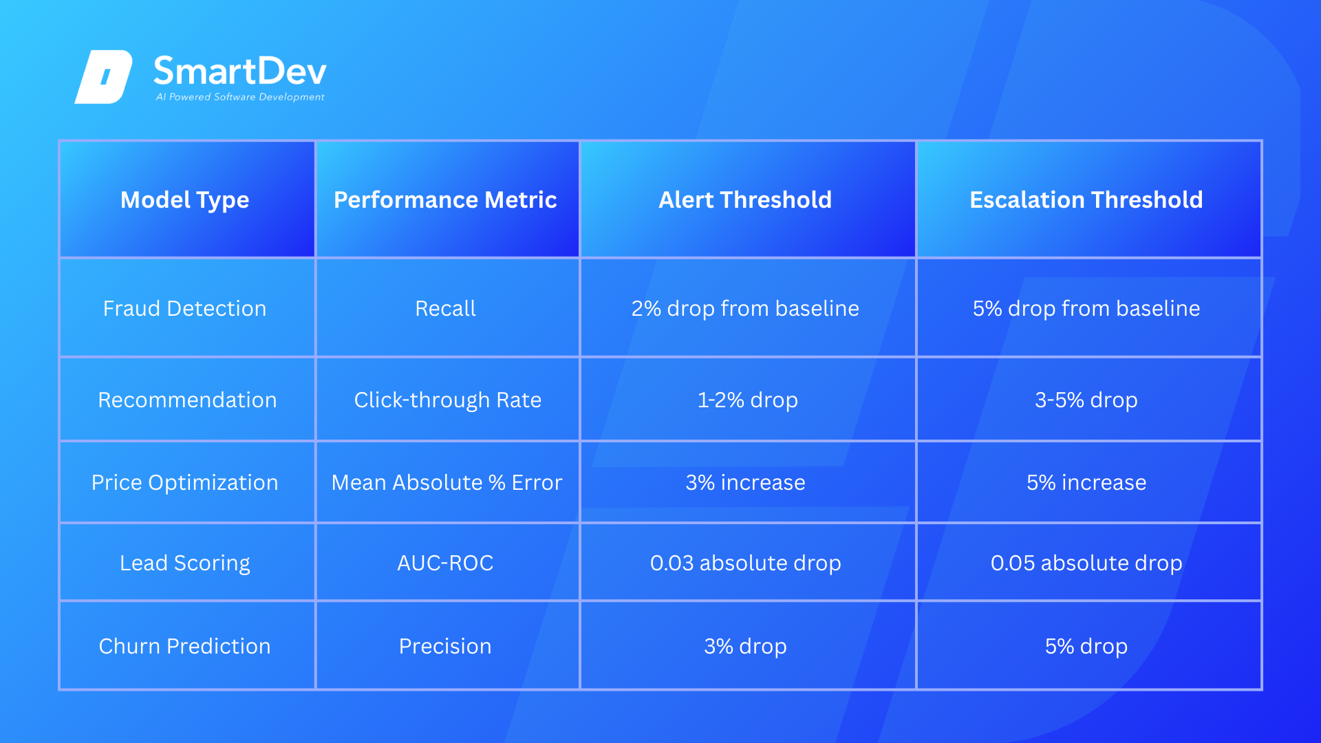
Practical thresholds for common scenarios: 

 

Step 3: Deciding When to Retrain – ML Retraining Schedule Strategies 

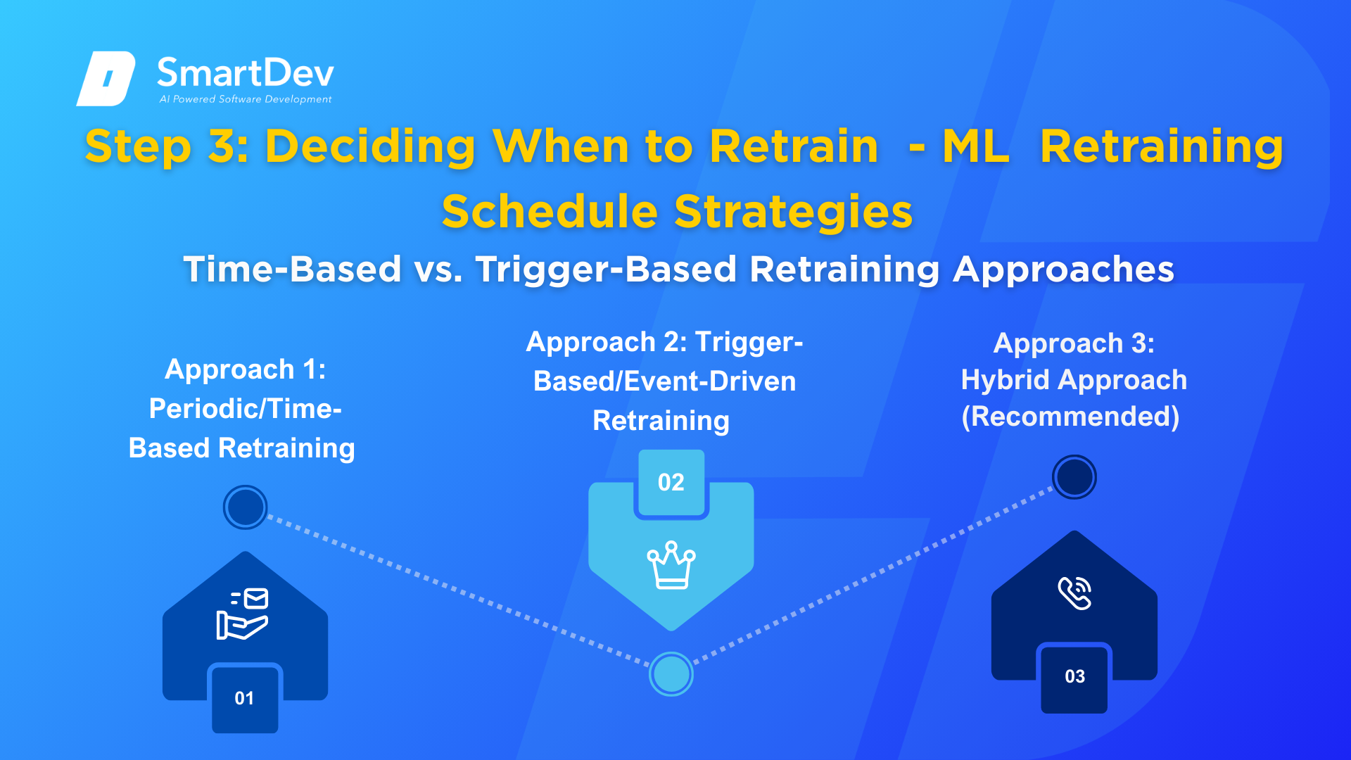
Time-Based vs. Trigger-Based Retraining Approaches 

When a drift is detected, you face a critical decision: How will you decide when to actually retrain? This is where your ML retraining schedule strategy becomes essential. 

Approach 1: Periodic/Time-Based Retraining 

Simple approach: Retrain a fixed schedule: daily, weekly, monthly, quarterly. 

When to use: 

• Models where data changes predictably (e.g., daily demand forecasting) 

• Systems with sufficient compute resources to handle frequent retraining 

• Production environments where you have adequate testing and deployment infrastructure 

• Models where gradual adaptation is important (recommendation systems) 

Implementation: 

• Daily retraining: Typically for high-frequency trading, real-time bidding, or other time-sensitive applications 

• Weekly retraining: Sweet spot for many systems; catches drift quickly without excessive resource consumption 

• Monthly retraining: For slower-changing systems or resource-constrained environments 

Pros: 

• Simple, predictable, easy to schedule 

• Gradually adapts to gradual data changes 

• Doesn’t require sophisticated drift detection 

Cons: 

• Wastes resources retraining when model is performing well 

• May be too frequent or not frequent enough depending on actual drift rate 

• All-or-nothing approach doesn’t differentiate between severe and minor drift 

Approach 2: Trigger-Based/Event-Driven Retraining 

More sophisticated approach: Monitor drift signals; retrain only when thresholds are exceeded. 

When to use: 

• Models where drift occurs unpredictably (concept drift) 

• Resource-constrained environments where you can’t afford frequent retraining 

• Production systems where unnecessary retraining creates deployment risk 

• Models where you want responsive adaptation to sudden changes 

Implementation: 

• Primary trigger: Performance metric drops below threshold 

• Secondary trigger: Data distribution significantly changes (PSI > threshold) 

• Tertiary trigger: External events (major competitor product launch, regulatory change, seasonal transition) 

• Include minimum retraining interval (e.g., “don’t retrain more than once per week” to avoid constant churn) 

Pros: 

• Efficient, only retrains when necessary 

• Responds quickly to sudden drift 

• Reduces deployment risk from unnecessary retraining 

• Lower resource consumption 

Cons: 

• Requires sophisticated monitoring 

• Can miss gradual drift if thresholds are set too high 

• May have lag between drift occurring and retraining triggering 

• False alerts can trigger unnecessary retraining 

Approach 3: Hybrid Approach (Recommended) 

Most production systems benefit from combining approaches: 

• Baseline schedule: Periodic retraining on fixed schedule (e.g., weekly) 

• Accelerated triggers: Additional retraining triggered if thresholds exceeded 

• Throttling: Minimum interval between retraining attempts prevents excessive churn 

This hybrid approach gives you stability from predictable retraining plus responsiveness to genuine drift. 

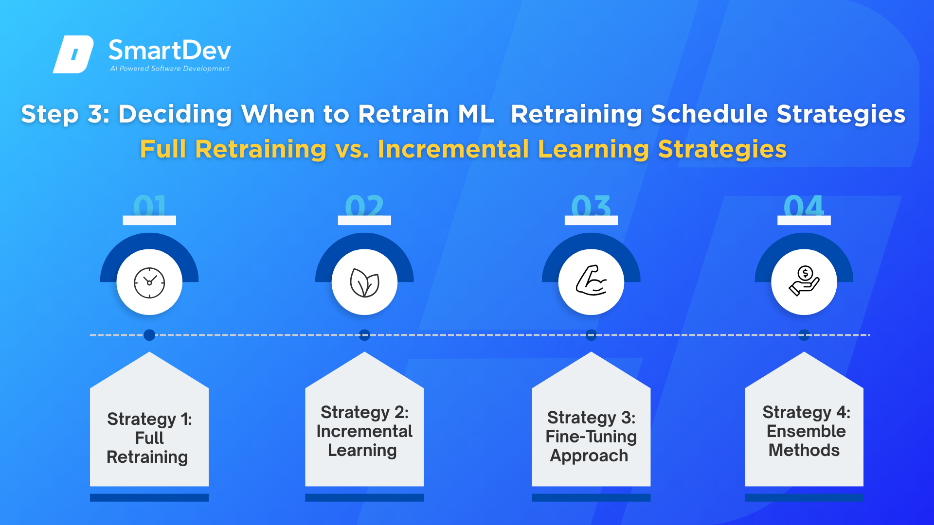
Full Retraining vs. Incremental Learning Strategies 

Once you’ve decided retraining is needed, the next question: Should you rebuild the entire model from scratch, or incrementally update it? 

Strategy 1: Full Retraining 

Complete models rebuild, delete old models, train new models on all historical data plus recent data, and deploy new models. 

When to use: 

• Significant concept drift requiring fundamental model changes 

• Less frequent retraining (quarterly, monthly, or when triggered by major drift) 

• When you have sufficient compute resources 

• When model quality is critical and you want no shortcuts 

Implementation: 

• Collect training data from entire historical period plus recent period 

• Retrain using same features, algorithms, and hyperparameters as original 

• Evaluate new model comprehensively before deployment 

• Allow 1-24 hours for training depending on data volume and model complexity 

Data sampling considerations: 

• Should you use all historical data or just recent data? 

• Best practice: Use all historical data to maintain learned patterns, but weight recent data higher 

• Example: Use data from past 12 months but weight last 3 months at 2x importance 

• Prevent “catastrophic forgetting” where model forgets patterns learned from historical data 

Pros: 

• Comprehensive learning from all available data 

• Can accommodate model architecture changes 

• Easier to understand and debug 

• Standard approach that works well 

Cons: 

• Computationally expensive for large datasets 

• Long retraining time limits frequency 

• Deployment risk-complete replacement can break things 

• Doesn’t efficiently handle incremental changes 

Strategy 2: Incremental Learning 

Update model using only new data: take existing model, refine it using recent data. 

When to use: 

• Frequent retraining requirements (daily or multiple times daily) 

• Resource-constrained environments 

• Gradual data changes requiring continuous adaptation 

• Streaming data scenarios 

Implementation: 

• Start with existing model weights 

• Train on recent data (typically last 7-30 days) 

• Update model parameters without resetting to random initialization 

• Deploy updated model 

Sampling strategy: 

• Balanced sampling: Mix recent correct predictions with recent errors 

• Typical ratio: 70% recent data, 30% recent error cases 

• Prevents “catastrophic forgetting” where model forgets historical patterns while learning new patterns 

• Stratified sampling: Ensure representation across important segments 

• Particularly important for classification with class imbalance 

• Example: If minority class represents 1% of data, ensure 1% of training batch is minority class 

Risk mitigation: 

• Regularization: Add L1/L2 regularization to prevent large parameter changes 

• Learning rate reduction: Use lower learning rates than initial training 

• Periodic full retraining checkpoints: Every 4-8 weeks, do a complete full retraining 

Pros: 

• Fast, can run frequently 

• Lower computational cost 

• Gradually adapts to changing data 

• Good for streaming scenarios 

Cons: 

• Risk of catastrophic forgetting 

• Less comprehensive learning from historical patterns 

• Can accumulate errors over time 

• Less flexible-harder to change model architecture 

• Requires careful implementation to avoid degradation 

Strategy 3: Fine-Tuning Approach 

Hybrid approach: Keep early model layers frozen, only retrain later layers. 

Use case: You’ve trained a deep neural network; the early layers have learned general patterns. Recent data changes affect later specialized layers. You can retrain just the later layers on recent data while keeping general pattern learning intact. 

Implementation: 

• Freeze early N% of layers 

• Retrain final layers on recent data 

• Balance regularization to prevent degradation of frozen layers’ learning 

Strategy 4: Ensemble Methods 

Train multiple models on different data subsets, combine predictions for robustness. 

Use case: You want to gradually retire from old models and introduce new ones without sudden transitions. 

Implementation: 

• Maintain ensemble of 2-3 models of different ages 

• Weight recent models more heavily 

• Gradually decrease weight of old models as they degrade 

• Replace oldest model when newest model proves stable 

Step 4: Implementing Automated Retraining Pipelines 

Building Production-Grade ML Retraining Workflows 

Successful production of AI maintenance requires automation. Manual retraining is too slow, too error-prone, and too expensive for production systems. 

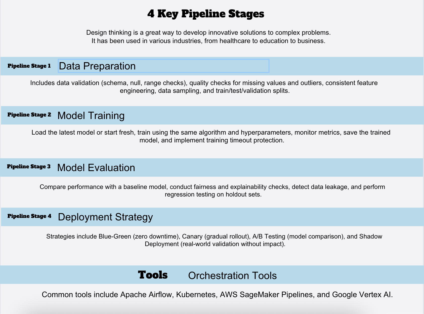
Pipeline Stage 1: Data Preparation 

First stage: get data ready for training. 

Components: 

• Data validation: Schema validation (expected fields, data types), null checks, range validation 

• Data quality checks: Identify and handle missing values, outliers, data quality issues 

• Feature engineering: Apply same transformations as original training pipeline 

• Data sampling: Apply sampling strategy (recent data weighting, stratification, etc.) 

• Train/test/validation split: Typically, 60-20-20 or 70-15-15 split using time-based or random splitting 

Implementation tools: 

• Great Expectations: Data quality and validation framework 

• TensorFlow Data Validation (TFDV): Statistical validation and schema checking 

• Custom Python scripts: For domain-specific transformations 

• dbt: For complex data pipelines and transformations 

Pipeline Stage 2: Model Training 

Training stage: Build the model using prepared data. 

Components: 

• Load latest model (if incremental learning) or start fresh (if full retraining) 

• Train on prepared dataset using same algorithm and hyperparameters 

• Monitor training metrics for divergence (training loss not decreasing indicates problem) 

• Save trained model with metadata (training date, data used, hyperparameters) 

• Training timeout protection: Automatically abort training if taking too long 

Implementation tools: 

• MLflow: Experiment tracking, model versioning 

• Weights & Biases: Training monitoring and experiment management 

• Custom training scripts: Using TensorFlow, PyTorch, XGBoost, scikit-learn 

• Cloud training services: AWS SageMaker, Google Vertex AI, Azure ML 

Pipeline Stage 3: Model Evaluation 

Evaluation stage: Validate a new model before deployment. 

Critical components:

1. Performance comparison:

• Compare new model’s metrics against current production model 

• Requirement: New model must meet minimum performance threshold 

• Example: “Deploy only if accuracy ≥ 0.92 AND F1-score ≥ 0.88” 

• Never deploy model that underperforms baseline 

2. Fairness evaluation:

• Check for demographic parity across important segments 

• Ensure fairness metrics haven’t degraded 

• Particularly critical for high-stakes models (lending, hiring, criminal justice) 

3. Explainability checks:

• Verify model decisions remain explainable 

• Check feature importance hasn’t changed dramatically 

• Identify if model relies on new suspicious features 

4. Data leakage detection:

• Verify model isn’t accidentally using future information 

• Check for dependencies on test data 

• Confirm features are available at prediction time 

5. Regression testing:

• Test on holdout test sets from training period 

• Verify performance on historical scenarios still works 

• Ensure model still handles edge cases

Manual review triggers: 

• Model rejected by automated checks 

• New features used in training 

• Training dataset size dramatically different 

• Training process took much longer than usual 

Pipeline Stage 4: Deployment Strategy 

Once evaluation passes, how to safely get the model into production? 

Option 1: Blue-Green Deployment 

• Maintain two identical production environments (blue and green) 

• Deploy new model to inactive environment (green) 

• After thorough testing, switch traffic to green 

• Keep blue as instant rollback 

Pros: Zero downtime, quick rollback
Cons: Requires duplicate infrastructure, higher cost 

Option 2: Canary Deployment 

• Deploy new model to small % of traffic initially (e.g., 5%) 

• Monitor canary performance vs. current model 

• Gradually increase traffic if metrics look good (5% → 20% → 50% → 100%) 

• Automatic rollback if metrics degrade 

Pros: Limited exposure to issues, real-world validation
Cons: Complex monitoring, slower rollout 

Option 3: A/B Testing 

• Run new model in parallel with current model for percentage of traffic 

• Statistically compare performance 

• Deploy whichever performs better 

Pros: Rigorous comparison, clear winner
Cons: Double resource consumption, slower decision 

Option 4: Shadow Deployment 

• Run new model in production but don’t use predictions 

• Capture predictions for offline comparison 

• Deploy if performance looks good 

Pros: Real-world validation without customer impact
Cons: Double resource consumption, no real-world feedback on decisions 

Orchestrating Automated Pipelines 

How to automate entire workflow: data preparation → training → evaluation → deployment? 

Tool: Apache Airflow 

Workflow orchestration tool designed for data pipelines. 

Configuration: 

• Schedule retraining: “Weekly on Monday at 2 AM” 

• Dependencies: Don’t start training until data prep succeeds 

• Notifications: Alert engineers if any stage fails 

• Retry logic: Retry failed tasks up to 3 times before alerting 

Tool: Kubernetes 

Container orchestration for scalable retraining. 

Configuration: 

• Define training job as Docker container 

• Kubernetes scheduler runs training containers with specified compute resources 

• Auto-scaling: Run multiple training jobs in parallel for large datasets 

• Integration with Airflow or other schedulers for orchestration 

Tool: Cloud-Native Pipelines 

AWS SageMaker Pipelines, Google Vertex AI Pipelines, Azure ML Pipelines provide pre-built solutions. 

Advantages: 

• Integrated with model registry and deployment 

• Automatic experiment tracking 

• Built-in monitoring and logging 

• Handles infrastructure provisioning 

Practical Retraining Pipeline Example 

Concrete implementation for e-commerce recommendation system: 

1. TRIGGER

• Daily at 3 AM (off-peak) 

• OR immediately if click-through rate drops 3% 

2. DATA PREPARATION (runs 3-4 AM)

• Query last 30 days of user interactions 

• Remove invalid sessions, bots, test users 

• Apply feature engineering (user age group, product category, time since last purchase) 

• Sample to 10M interactions (balanced sampling: 70% random, 30% low-score interactions) 

3. TRAINING (runs 4-6 AM)

• Load existing recommendation model 

• Apply incremental learning with learning rate 0.001 

• Train on prepared data for 2 hours max 

• Save new model with metadata 

4. EVALUATION (runs 6-6:30 AM)

• Compare new model AUC-ROC vs. current production (0.758) 

• Requirement: New model must be ≥ 0.750 

• Compare click-through rate vs. expected (2.1%) 

• Requirement: New model must achieve ≥ 2.05% CTR 

5. DEPLOYMENT (runs 6:30-7 AM if evaluation passes)

• Canary: Send 5% of traffic to new model 

• Monitor for 30 minutes 

• If CTR > 2.09%, increase to 20% 

• If CTR > 2.10%, increase to 100% 

• If CTR < 2.06%, automatic rollback to previous model 

6. MONITORING

• Daily: Calculate CTR, feature drift scores 

• Weekly: Human review of model performance trends 

• Trigger new cycle if CTR drops 2% 

Step 5: Managing Retraining Data and Avoiding Common Pitfalls 

Data Selection and Sampling for Production Retraining 

One of the most common mistakes in production model maintenance: using wrong data for retraining. 

Pitfall 1: Using Too Much Old Data 

Scenario: You have 5 years of historical data. You retrained using all 5 years of data plus recent month. 

Problem: Ancient patterns (from 5 years ago) may no longer be relevant. Your model learns outdated patterns and performs worse on recent data. 

Solution: 

• Use recent historical data (typically 1-2 years of recent data) 

• For models in rapidly changing environments (fashion, current events), use only 3-6 months 

• For stable models (credit risk, physics simulations), can use 3-5 years 

Pitfall 2: Over-Weighting Recent Data 

Scenario: You retrain using only last 30 days of data for a recommendation model. 

Problem: Temporary patterns and noise in last 30 days can dominate. You lose learned patterns about longer-term user behavior. 

Solution: 

• Balance recent and historical data 

• Typical approach: Use last 2 years of data but weight last 3 months at 2x importance 

• Prevents catastrophic forgetting while adapting to recent patterns 

Pitfall 3: Not Accounting for Class Imbalance 

Scenario: Your fraud detection model catches fraud in 0.5% of transactions. You train on balanced data (50% fraud, 50% legitimate). 

Problem: Model is vastly overconfident about fraud probability. Deployed model generates excessive false alerts because it thinks fraud is 50% likely instead of 0.5% likely. 

Solution: 

• Maintain class imbalance in training data matching production distribution 

• Use resampling/reweighting if you need balanced training but apply calibration before deployment 

• Monitor predicted probability distributions-they should match observed rates in production 

Pitfall 4: Data Quality Degradation 

Scenario: Production data becomes messier over time (missing values increase, outliers appear). 

Problem: Model trained on degraded data learns to expect degraded data. When data quality improves (or worsens further), model performance degrades. 

Solution: 

• Validate data quality before training 

• Apply same data cleaning as original pipeline 

• Monitor data quality metrics continuously 

• Alert when data quality degrades 

Pitfall 5: Data Leakage 

Scenario: Your model for predicting next-month sales includes current-month sales figures in features. 

Problem: Works great in training but fails in production because current month’s sales aren’t available when making predictions. 

Solution: 

• Document exactly what information is available at prediction time 

• Remove any features that violate availability constraints 

• Regularly audit for data leakage 

Handling Label Delays and Feedback Loops 

Production models often face significant label delays: ground truth becomes available weeks or months after predictions. 

Challenge: How to detect model degradation when you can’t directly measure performance? 

Solution 1: Use Proxy Metrics 

While waiting for labeled data: 

• Monitor data distribution metrics (PSI, feature drift) 

• Monitor prediction distributions 

• Monitor business metrics (click-through rate, conversion rate, revenue) 

When labels eventually arrive: 

• Verify proxy metrics correctly predicted actual degradation 

• Calibrate which proxy metrics are most predictive 

Solution 2: Active Learning 

Selectively collect labels for uncertain predictions: 

• Identify predictions where model is least confident 

• Manually label subset of these predictions 

• Retrain on labeled subset to improve uncertain areas 

Cost: Manual labeling is expensive but covers most important cases. 

Solution 3: User Feedback as Labels 

Some applications naturally generate feedback: 

• E-commerce: User clicks on recommendations 

• Search: User clicks search results 

• Ads: User clicks ads 

• Music: User likes/dislikes songs 

Use this feedback as pseudo labels for model retraining. Requires caution: feedback bias can affect training. 

Step 6: Governance and Long-Term AI System Upkeep 

Technical excellence isn’t sufficient for long-term AI system upkeep. You also need governance frameworks to ensure responsible, sustainable model management. 

Governance Component 1: Model Registry and Versioning 

Every model should be versioned and tracked: 

Minimum information: 

• Model version identifier (v1.0, v1.1, v2.0) 

• Training date and data period 

• Performance metrics (accuracy, F1, AUC, etc.) 

• Features used 

• Algorithm and hyperparameters 

• Training code version (Git commit hash) 

• Training environment (Python version, library versions) 

• Deployed date and production performance 

Tools: 

• MLflow Model Registry 

• Hugging Face Model Hub (for NLP models) 

• Cloud-native registries (AWS SageMaker, Google Vertex AI) 

Governance Component 2: Change Management and Approval 

Never deploy model changes without review: 

Process: 

1. Model training completes 

1. Automated evaluation checks run 

1. Model flagged for human review if: automated checks fail, new features used, performance changed significantly 

1. Senior ML engineer or domain expert reviews and approves 

1. Deployment proceeds only with approval 

1. Change documented in model registry 

Approval criteria: 

• Performance meets minimum threshold 

• Fairness metrics acceptable 

• No data leakage 

• Training code reviewed 

• Deployment risk assessed 

Governance Component 3: Performance Monitoring and Alerting 

Continuous monitoring post-deployment: 

Monitored metrics: 

• Primary performance metrics (accuracy, AUC, etc.) 

• Secondary metrics (fairness, explainability) 

• Data quality metrics 

• Model stability metrics 

Alert escalation: 

• Green: Metric stable and within expected range 

• Yellow: Metric degrading but still acceptable (2% below baseline) 

• Red: Metric critically degraded (5%+ below baseline) → automatic escalation and emergency retraining review 

Governance Component 4: Documentation and Runbooks 

Clear documentation prevents mistakes and enables faster incident response: 

Model Card (document for each model): 

• What problem does this model solve? 

• Performance characteristics: Accuracy, fairness, limitations 

• Intended use: Which use cases are model appropriate for? 

• Retraining frequency: How often does the model get retrained? 

• Retraining triggers: What conditions trigger retraining? 

• Known limitations: Where does a model perform poorly? 

• Fairness considerations: How do models perform across demographic groups? 

• Data Requirements: What data needs to be retrained? 

Operational Runbooks: 

• “Model performance degradation: suspected drift” → steps to investigate and resolve 

• “Emergency model retraining” → fast-track process for urgent retraining 

• “Model rollback procedure” → how to revert to previous version if problems emerge 

• “Data quality issue detected” → notification and remediation steps 

Governance Component 5: Incident Tracking and Continuous Improvement 

When problems occur, learn from them: 

Incident tracking: 

• Date and severity (critical, high, medium, low) 

• Symptoms: What went wrong? 

• Root cause: Why did it happen? 

• Resolution: What was done? 

• Prevention: How can we prevent this in future? 

Example incident: 

• Date: March 15, 2024 

• Severity: High 

• Symptom: Fraud detection model missed spike in fraud on March 14 

• Root cause: New fraud pattern not in training data; concept drift 

• Resolution: Manual retraining on recent fraud data; deployed new model 

• Prevention: Implement daily drift detection using prediction distribution shift metrics 

Continuous improvement from incidents: 

• Share learnings across teams 

• Adjust thresholds based on incidents 

• Improve monitoring based on what incidents revealed 

• Update training procedures 

Sustainable Production ML through Continuous Monitoring and Maintenance 

Model drift is not an exception; it’s the norm. Without rigorous AI model drift detection, systematic model performance monitoring, disciplined ML retraining schedule execution, and comprehensive production of AI maintenance governance, your deployed models inevitably degrade into mediocrity. 

The organizations that maintain competitive advantage through AI are not those with the best initial models. They’re those with the best production model management. They’ve built systematic processes for: 

1. Continuous monitoring that tracks whether models continue delivering value 
2. Automated drift detection that identifies performance degradation early 
3. Intelligent retraining that responds systematically to degradation 
4. Governance frameworks ensuring responsible, sustainable AI operations 
5. Long-term partnerships with vendors who understand that delivery is the beginning, not the end 

This comprehensive guide provides a roadmap. The next step is implementation: starting with your highest-priority production models, establishing basic monitoring, implementing drift detection, automating retraining, and gradually building the governance practices that make AI system upkeep systematic and sustainable. 

Your models’ ability to remain accurate, fair, and valuable over months and years depends entirely on the production maintenance systems you build today. Begin with this framework. Adapt it to your specific needs. And commit to the ongoing discipline of keeping your production of AI systems healthy, accurate, and valuable for as long as they’re deployed.